| |
Blackjack Card Counting Studies
This page contains links to and explanations of several
charts which have been created with CVData and provide illustrations
of many Blackjack principles. Note: Some of these studies
are quite advanced. You do not need to understand these charts
to count cards. Below is a quick index of sections describing
the charts. Each section has one or more links to the chart
images.
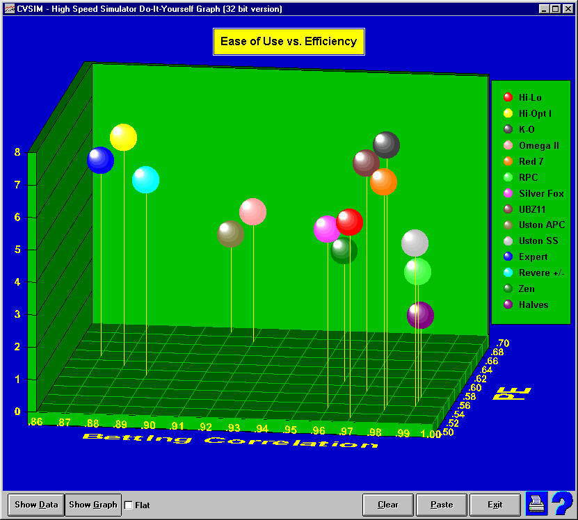
Ease of Use vs.
Efficiencies of Various Strategies
In an attempt to visually illustrate the differences in
ease of use and efficiencies between strategies, Ive created
a 3D Scatter Chart. The chart consists
of 14 balloons suspended above an x-z grid. The x-axis is
Betting Correlation. The z-axis is playing efficiency. The
string from each balloon intersects the grid at the BC and
PE for that strategy. The height of the balloon (y-axis) is
the ease of use of the strategy. Thereby, each balloon indicates
all three variables. The ideal system (impossible to obtain)
would be at the top, right, back. Note, the two strategies
in the center (Omega II and Uston APC), are very high PE,
Ace-Neutral strategies. If Ace side counts are kept for these
strategies, they would move substantially to the right placing
them closer to the ideal combination of efficiencies. However,
they drop in height as they become more difficult to use.
Be careful of the parallax problem. Balloons closer to the
front appear not to be as high as they are.
Advantage and
Units Won/Lost vs. True Count
The count is better for you at extremely high counts with
two esoteric exceptions (described at the end.) Ive attached
a combination chart which shows Advantage
and Units Won/Lost vs. True Count. The green area shows the
losses at negative values and gains at positive values. Of
course, the big gains and losses are at relatively low plus
or minus counts, because this is where the majority of hands
exist. The red line shows advantage. It is very smooth for
the majority of counts, but goes wild at the very high and
low counts. This is despite the fact that this is a simulation
of one billion hands and the data has been smoothed (with
a quadratic B-spline algorithm.) Problem is, there just arent
that many hands at the extreme counts and the variance is
obscene. Of course, if you play long enough, you will experience
a few wild counts. Your results at those counts are essentially
random. Unfortunately, the human mind is more likely to remember
such events, even though they have no meaning. This is why
people watch X-files and other silly TV shows.
Esoterica
- 1. If you are playing single deck, and you and all
other players play without any variation whatever, then
certain wild TCs will only occur with certain dealt card
sequences. This will result in automatic wins or losses
at specific extremely high or low counts. The odds of running
into this situation are approximately zero.
- 2. If you are side-counting Aces and there are none
left, youve got a problem with a high count.
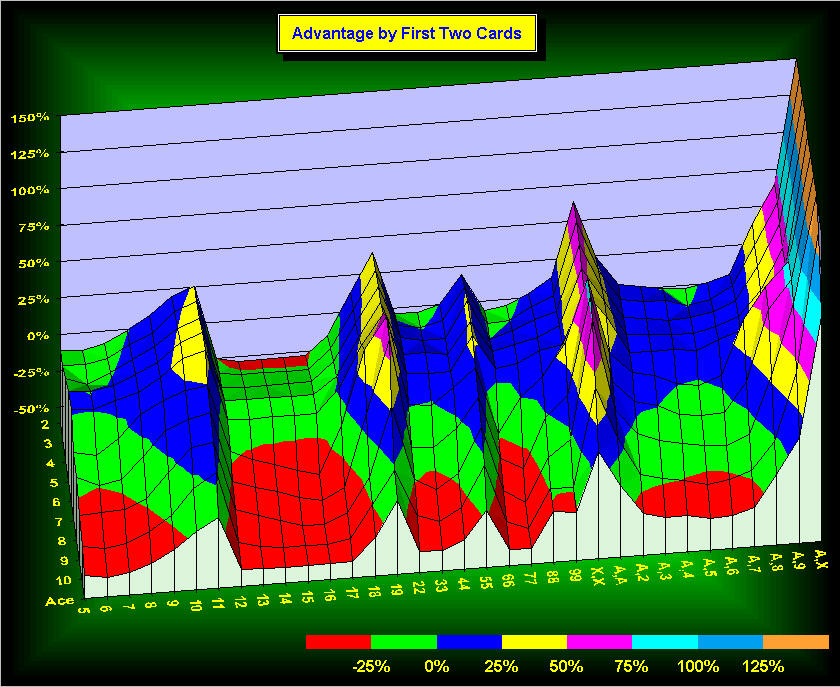
Advantage by Type
of Hand
I've been experimenting with topology maps in an attempt
to better show statistics by type of hand. The attached Advantage
Surface Chart shows advantage for the various first two
cards. X-axis is type of hand (all hard hands, soft hands
and pairs). Z-axis is dealer up card. Y-axis is eventual advantage
given six deck, Hi-Lo, 1-8 spread.
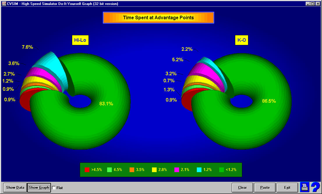
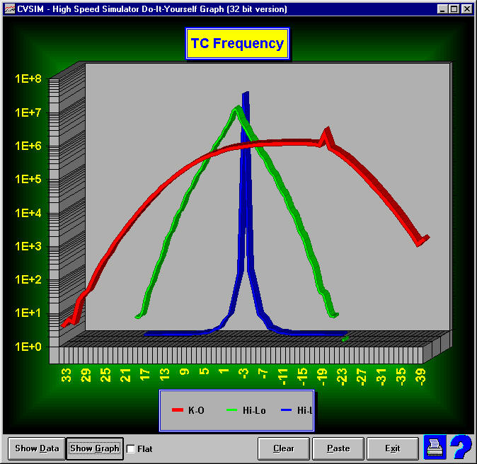
Time Spent in
Advantage Situations Balanced vs. Unb.
Comparing the percentage of time that two systems indicate
specified advantages is problematic because the counts are
not continuous. Different systems result in different levels
of advantage percentage. However, I took a shot at it:
The first chart
displays the time spent at certain advantages for K-O and
Hi-Lo.
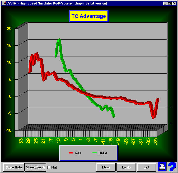
The second chart
shows the advantage at each count (Running Count for
K-O and True Count for Hi-Lo.)
The third chart
shows the frequency of hands at each count. Here, the red
and green are charted using a logarithmic scale. The blue
ribbon in the back is the same data as the green ribbon plotted
with a standard scale. It is there to show why I had to use
a logarithmic scale and to show the huge number of hands at
a TC of zero in a system that truncates instead of rounds.
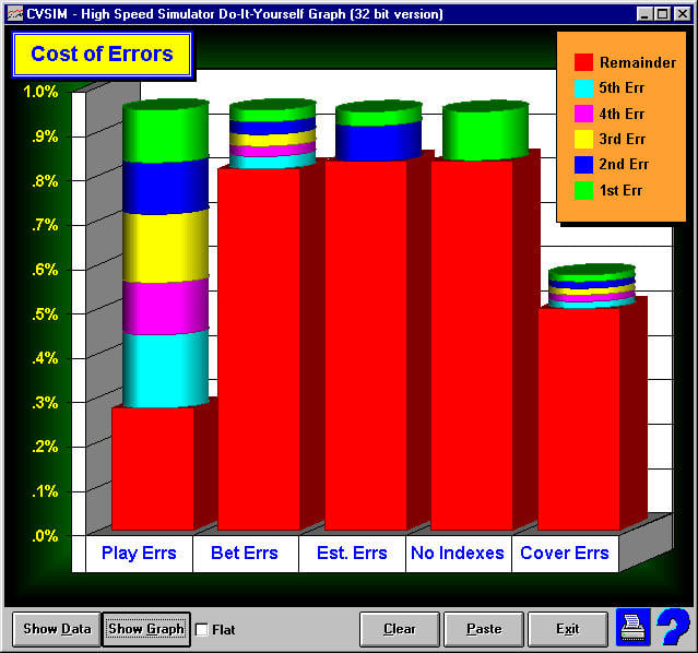
Cost of Errors
The Cost of Errors Chart is an
attempt to show the cost of various types of errors. Five
columns are provided using data from five multi-deck, multi-player
sims. The height of the columns represents advantage.
- Column 1 displays the effect of playing errors. The
total height of the column represents the advantage with
no errors. The green segment indicates the penalty resulting
from one error per hundred hands. The blue section is the
additional penalty of another error per hundred. And on
through five errors. The red pedestal is the advantage with
a 5% error rate. The errors are serious; but not idiotic.
Insure is reversed, surrender is reversed, split or double
is changed to hit, hit and stand are reversed. But, a hard
18 up is never hit, an eleven down is never stood, and a
double or split is never taken when it shouldn't.
- Column 2 displays the effect of betting errors for
a non-cover bettor. Again, succeeding circular slices of
the bar show the effect of errors. The player is spreading
1 to 8. Errors are: if should be a one bet, bet two; if
should be a two, bet three; if should be a three through
eight, but two.
- Column 3 displays the effect of miss-estimating the
remaining cards for TC calculation. The green shows the
effect of a 10% error and the blue shows the additional
effect of an additional 10% error.
- Column 4 shows the effect of using no indexes at all.
The green section is the penalty when using perfect BS vs.
-10 to +10 indexes. The count is still used for betting
purposes.
- Column 5 is the effect of errors for a cover-bettor.
The betting is very conservative not allowing large increases
or decreases, no increases after losses, no decreases after
wins and no change after pushes. The error scenario is too
complex to explain here. (OK, Im too lazy.)
I did not include a column for flat betting, because there
wouldnt be one. Youd lose all of your advantage.
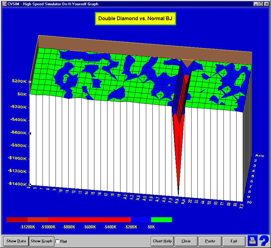
Double Diamond Blackjack
A question was raised as to the advantage of a new game
called Double Diamond Blackjack. This game pays extra on a
Diamond BJ, but less on other BJ's. Also, several other fancy
rules are added. The problem with such a game is the huge
penalty of reducing the BJ payoff. I've created a Surface
Area Chart which displays the difference in winnings between
a normal single deck game and a game like Double Diamond (DD).
The DD game I used was 6 card charlie, 5 card 2:1, Diamond
BJ pays 2:1, Normal BJ pays even, but is automatic win, Double
on any number of cards even after splits. The chart has all
two card hand types on the x-axis, dealer upcard on the y-axis
and difference in winnings on the z-axis. The z-axis is winnings
on the Diamond game minus winnings on a normal game.
Looking at the chart, the games are equal where the blue
and green meet. Green is a slight advantage for DD, red is
a serious disadvantage for DD. The green/blue splotchiness
is due to the small number of hands run (160,000,000). It
indicates that the variance at that number of hands is actually
greater than the difference in results between the two games.
The solid green with upcard combinations totalling 5, 6, 7
and 8 indicates a very slight gain in using the DD rules.
This is due to the gain from double on any number of cards,
6 card charlie, and 5 card 21. The huge slice through the
stack shows the loss due to most BJ's paying even money. This
is somewhat less at BJ vs. Ace because of the BJ automatic
win rule.
The point of the chart is to show the enormous penalty
of the BJ rule change versus the very slight gains by the
oddball rules.
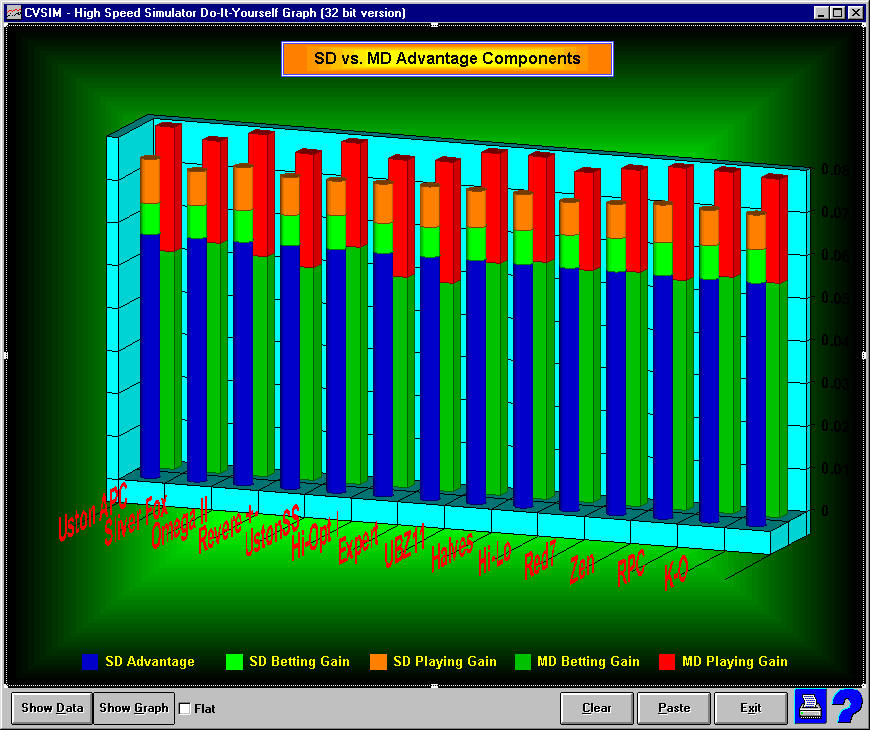
Components of Advantage
This chart provides two rows of Stacked
Bars. There are 14 pairs of bars representing the advantages
that can be gained using various strategies according to Griffin
calculation techniques. The y-axis (advantage) is not quantified
as it is relative. The rectangular columns in the back row
indicate the relative gains when playing multi-deck. The dark
green signifies gain from betting and the red indicates gain
from using indexes. A 1-8 spread is assumed. The circular
columns in the front row indicate the relative gains when
playing single deck. A 1-2 spread is assumed. Here, three
components are displayed. Again, betting and playing gain
are shown. The, additional, blue segment indicates the gain
from playing SD vs. MD.
So, what does this chart illustrate? Nothing new; but
a few concepts that should be kept in mind:
- Playing gain is equal to or more important than betting
gain in SD as opposed to MD where betting gain is substantially
more important. However, both are important in MD.
- Spread can make up for the loss in MD advantage, or
for the pessimist, spread is necessary to make up for the
loss in MD advantage.
- The differences between systems are dwarfed by the
difference in spread. That is, we spend altogether too much
time thinking and debating about which system is best and
not enough time talking about how to maximize the spread
without getting tossed. This is the simple point of the
chart.
Disclaimers: No simulations were run. Results are calculated
from Griffin formulae. Side counts, number of indexes and
cover plays are ignored. PE calculation is questionable for
unbalanced counts.
First Base Penalty
For some time, we have been aware that it is better to
sit at third base in single deck, face down games. Common
sense tells us that we get to see more cards and can make
better playing decisions. In an extreme case (seven players),
the advantage difference between seats 6 and 7 is about 0.05%.
You lose another .05% per seat as you move toward first base.
However, the difference in advantages between first and second
seat is much worse. First seat can be as much as .16% worse
than second seat. As this is a severe penalty, I decided to
take a look. First, I looked at the winnings by true count.
I created a chart which shows the winnings for first seat
and second seat by true count. [link]
The chart shows that the winnings are identical for all counts
below 4. But, at a TC of 4, second seat does better. At 5-8,
better and better. After that,. It evens out. OK, we now know
that there is something about these particular counts that
we should examine. I then decided to look at hand types. I
took the winnings for the second seat and broke them up into
an array of all possible two card hands vs. dealer up cards.
This is an array of 330 values. I also created the same array
for the second seat. I subtracted the second array from the
first array and charted the remainders. The result is a combination
surface area/contour chart that indicates the hands where
the first seat has a problem. [link]
Eureka! First seat has a serious problem with two tens against
a 3, 4, 5 and 6. Tens vs. 6 is particularly severe. All other
hand results are about the same. Common thinking would have
expected many differences along the lines of the Illustrious
18.
So, we have a problem with 10s against 3-6 at TCs of
4-8. Guess what, the indexes for splitting tens at 3-6 are
4-8 (Hi-Lo.) So, why is there a major problem with splitting
tens in seat one? Well, if you think about it, there is a
quirk in seat one. Remember, we are playing SD, face down,
seven seats. That means, two rounds. Only round two is important
as that is where you are betting. To split tens, you must
have two tens and the dealer must have a low card. If you
are sitting at seat one, the only cards that you can see after
the start of the round are two high cards and one low card.
This means that the playing count will now be the count at
the start of the round minus 1. If the round starts at a TC
of +3, any seat has the possibility of splitting tens against
a 3. That is, any seat except for seat one. Seat one cannot
because the count will always be one less than the count at
the start of the round or +2. 9% of the time, you will start
round two at a true count of +3. 2.74% of the time, you will
start at a true count of +4. This means that 6.26% of the
time, every player has the possibility of splitting tens against
a 6 in the second round, except for the player in seat one.
(26% of all gain is in round two at a starting TC of +3 in
this example.) The same holds for the other ten split opportunities,
at reduced percentages. Therefore, seat one, and only seat
one, has an automatic reduction in opportunity.
By the way, if you go through the same process between
other seat pairs, you get the charts that you would expect.
That is, the tens peak is muted and the other Illustrious
18 decisions start to poke out from the plane.
I dont consider this analysis complete and welcome comment.
Exact vs. Estimated
TC Calculation
This section summarizes sims of nine billion hands with
various methods of desk estimation. With the parameters that
I used, TC calculation using exact (to the card) deck
depth gave a .829% advantage and $17.29 win rate. When estimating
the number of decks, generally, the worse the method of estimation,
the lower your advantage, but the higher your win rate. This
is due to overbetting. To show where this overbetting occurs,
I chose a common method of deck estimation (287-312 cards=6
decks, 235-286=5 decks, etc.) and compared it to exact depth.
Advantage is .810% and win rate $17.32 (very slightly higher
than using exact remaining cards.) I created a chart showing
the average bet on the Y-axis and deck depth on the X-axis.
In general, average bet increases as deck depth increases
because there are more high TC's. The average bet increases
smoothly when TC calculation is performed with exact
remaining cards. However, the increase is lumpy when the remaining
decks are estimated. If you look at the chart (link is below)
you will see how the sloppy estimate shows lumps of higher
betting. The lumps increase in volume as deck depth increases
because of the higher percentage of large TC's. These lumps
in the graph signify the areas of overbetting. The area of
the largest lump is the area of highest risk.
CHART
Conclusions
The better your deck esitmation the smoother and more
accurate your betting, improving exposure to risk but not
income.
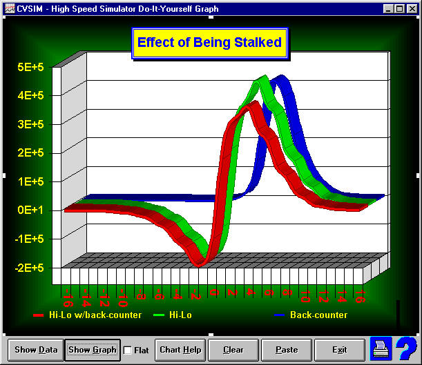
Effect of a Back-Counter
on your Play
Awhile back, I commented that Id leave a table if I thought
it was being stalked by a back-counter. Thought Id sim the
effect. Ran two sims. First sim had three players. BS players
in seats one and two and a Hi-Lo player in seat three. We
are interested in seat three. Second sim was the same, but
a fourth player Wonged in at a TC of +4 and left at the end
of the shoe. Again, we are interested in seat three. Six decks,
five deck penetration. Each player played 150 million hands
except the back-counter who played 13 million. The attached
ribbon chart (link below) graphs the winnings by TC for the
Hi-Lo player in each sim plus the back-counter. You will note
that the red ribbon (seat 3 in the second sim) and the green
ribbon (seat 3 in the first sim) run evenly through the negative
TCs. At about +3, the green player pulls ahead. That is,
the Hi-Lo player at the table with the back-counter won less
money on positive counts. Overall, he lost about 0.15% advantage.
FIRST CHART
- Winnings by TC.
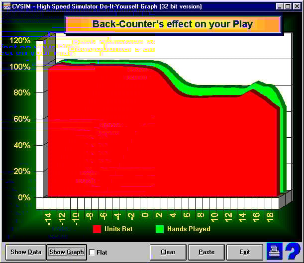
OK, where is the lost advantage? The second chart has
two series. The green series is the percentage of hands played
by seat three at the back-counters table of the hands played
by seat three at the back-counter-free table. The chart shows
that both seat three players played the same number of hands
at negative TCs, but at positive TCs, the player disturbed
by the back-counter played only 80% as many hands. This is
due to the back-counter eating cards in positive TC conditions.
So far, no surprise. However, there is another effect. The
red series on this chart shows dollars bet instead of hands
played. Again, the players at both tables bet the same per
TC at negative TCs. But, at positive TCs the drop-off in
units bet is more severe than the drop off in hands played.
Only 75% as many units are bet at high TCs. That is, the
average bet was lower at high TCs. Why is this? Well, the
Hi-Lo player was using camouflage play. The spread was 1-8
on both tables, but the player would never make large hand-to-hand
bet increases. Since the back-counters interference tended
to reduce the length of high TC consecutive hands, and reduced
the number of hands dealt per shoe in favorable situations,
the Hi-Lo player had fewer opportunities to win enough hands
in a row to pump his bet up to the optimum level.
CHART TWO
- Hands played and Units bet by TC
This shows an important point about running a sim exactly
as you would play. It is not enough to show a simple 1-8 spread
since realistic cover play may interact negatively with other
characteristics of the sim.
Note: When just looking at the overall advantage, 150
million hands is OK. But, when you break this down into smaller
groups of hands (e.g. by TC), then you have fewer hands per
situation and need more total hands to give good results.
However, there is a short-cut that was used here. All lines
were smoothed with a 12 facet cubic B-spline formula. This
takes information about neighboring data points (nearer points
count more than farther points) and adjusts all points to
produce a smoother graph. This requires several hundred million
calculations, but thats only seconds on a Pentium. If you
are looking for exact data, this is not valid. But, if you
are looking at trends, it is quite accurate and fast. To perform
this on a CVSIM chart, double-click on a series (e.g. group
of bars, a line, an area). The Format Series dialog box will
appear. Click on the Options tab. Then, select a Smoothing
formula at the bottom left. Click on Help to get information
on the options.
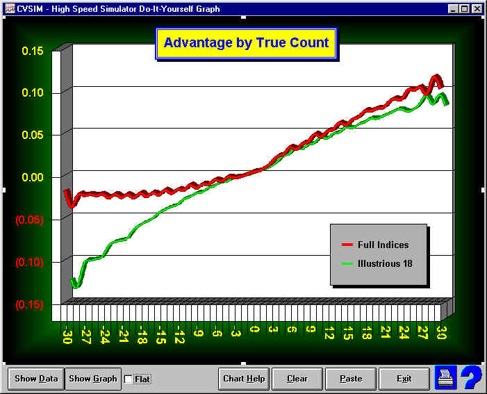
Advantage at Very
Low TC's
If you are using a huge number of indices, then your disadvantage
at very low counts is slight. You have the ability to alter
your play which makes up for part of your disadvantage. However,
these days, few people bother with the negative indices. If
you are using the Illustrious 18, then your advantage at very
low TCs drops precipitously. The attached
chart shows advantage by TC for two players at the same
table. One uses the Ill. 18 and the other uses a full set
of indices. Advantage at TCs below -14 barely changes for
the full index player. Advantage for positive TCs continues
to grow for both players. Does this mean that you should use
a full set of indices? No, very little money is bet at those
very low TCs.
Sim particulars: Single deck, three players, 1.6 billion
hands per player, four rounds per shuffle, SE at TC -30 was
.14. AO II was used as it has an excellent set of SD indices.
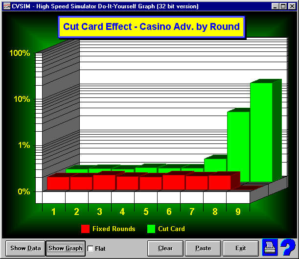
Cut Card Effect
Thought Id put together some charts to illustrate the
Cut-Card Effect. I created four charts from 2.6 billion single-deck,
basic strategy hands. About half of the hands were fixed at
eight rounds per deck and the other half dealt to a 75% penetration
(6 to 9 rounds.) The first simple
chart shows the advantage by hand depth. The red bars
show a even 0.2% advantage for the casino for all hand depths
when dealing a fixed number of rounds. The green bars show
the enormous increase in the casinos advantage in the late
rounds when dealing with a cut card. The advantage is so great,
that I had to use a logarithmic scale (0.2% to 14%). Fortunately,
there are not many hands dealt at the 14% casino advantage.
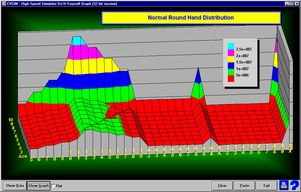
The following three charts each show hand dealt quantities.
Each chart has as its x-axis, all possible first two card
player combinations. The y-axis shows the dealer up-card.
The z-axis shows the number of incidents of each of the first
two player cards vs. dealer up card..
Chart I: The
first chart shows the normal distribution of hand types. That
is, the number of times that you will receive each of the
possible first two cards against each dealer up card.
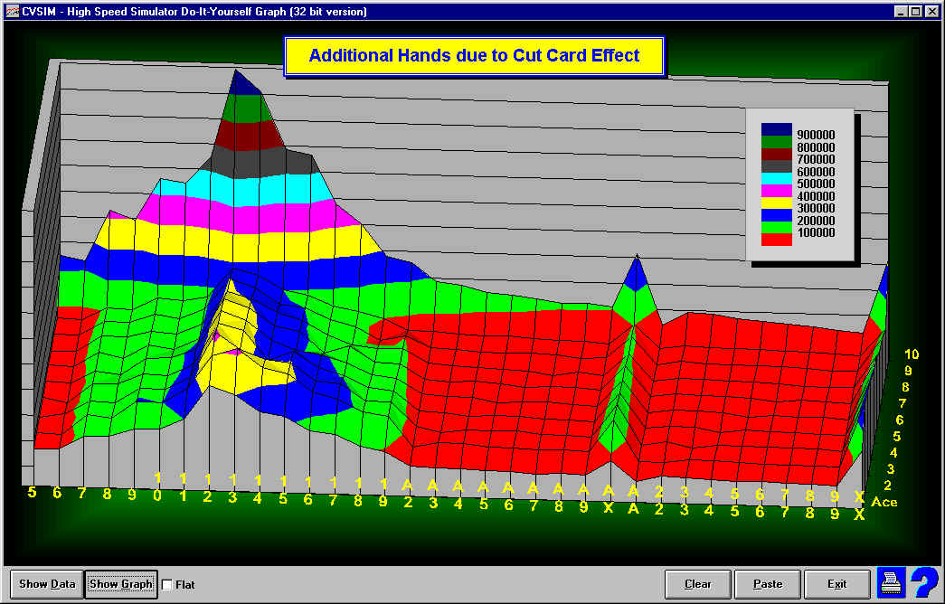
Chart II:
The second chart shows the distribution of hand types in the
last rounds when playing with a cut card. In this chart, there
exist more low cards since it is much more likely that you
will see additional rounds when large cards are dealt in the
earlier rounds.
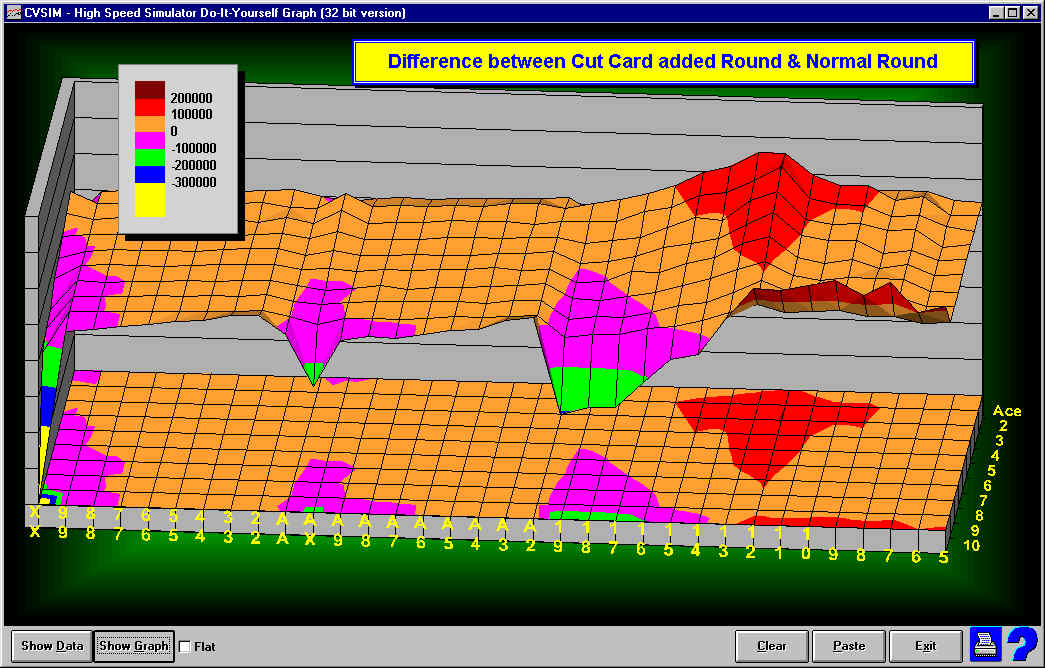
Chart III:
This is essentially the difference between the two previous
charts. It shows the delta between the normal distribution
of hands and the distribution of hands in the late rounds
when using a cut card. This is a surface area chart with a
projection of the colors to the base to more easily see the
problem areas. Red and orange areas show the types of hands
more likely to be seen in the late rounds. The chart shows
a substantial increase in stiffs, particularly against dealer
low cards. Also, more low hands (5-12) against a dealer ten.
There is a corresponding decrease in BJs, twenties, and 17-19
hands against good dealer up cards.
I also have an old
chart which shows the advantage at each of the above hand
types. It can be seen that most of the hands where we have
seen increases due to the cut-card effect are poor advantage
hands.
Of course, all that Ive shown with all of the above is
what was already known. The cut card adds hands when the deck
is lean in tens. So, does this mean that you should avoid
SD dealt to a fixed penetration. Yes, if youre playing BS.
But, if youre counting, its not so clear. Ive just started
working on those charts, and it appears that counting overcomes
the effect even in the late rounds. At least at the depths
at which Im currently testing.
The Effect of Number
of Players with Cover Betting
Normally, the number of players at a table has no effect
on your advantage. However, when cover betting, this can change.
I ran a total of five billion hands with cover betting as
follows:
- No increase in bet after loss
- No decrease after win
- No bet change after push
- Max increase or decrease two units
- No cover plays
- 1-8 Spread (1, 2, 4, 6, 8 at TC's of 1, 2, 3, 4, 5)
- I allowed bet reset to one unit at shuffle as not resetting
would clearly hurt a full table player.
- Five/six deck, strip rules
Advantages:
- 1 player: 0.60%
- 4 players: 0.45%
- 7 players: 0.33%
I created a Bet Size by TC Chart
for the three players. X-axis is TC, y-axis is average amount
bet (including double downs.) The red bars show the rapid
increase in average bet size for the head-on player. It nearly
matches the ideal. It drifts off very slightly at very high
TC's because there are slightly fewer DD's at high TC's. The
green and blue bars show the players' at fuller tables much
slower and smoother increase in average bet size as they have
more difficulty raising there bets quickly as high TC's occur
at lower hand depths. It also shows them overbetting at +1
and +2 as they couldn't lower bets as quickly as desired.
I tried small sims with various number of players and
no cover. There is no difference without cover. Also, the
effect of cover when playing head-on is negligible. I also
tried softening the cover by allowing a doubling or halving
of the bet and allowing bet increases after a lost split or
double and bet decreases after a won split or double. Didn't
appear to change the results much, but I need to make more
runs in that area.
The Effect of Cover
on Advantage by Penetration
I put together an Effect of Cover
chart to give some idea of the cost of various amounts of
cover betting. The results are from one half-billion round
sim. There were four players as follows:
Yellow: No cover Blue: No bet increases after a loss,
no decreases after a win; but reset to one unit after a shuffle
Green: Same as above but also no bet change after a push and
no jumping bets up or down by more than two units. Red: Same
as above but bet not reset to one after shuffle and Insurance
Cover. (index of 4 for a BJ, 3 for a twenty and 2 for other
hands.)
All players had a spread of 1-8. A two unit bet was allowed
at TC of +1 Which is earlier than in BJ Attack's sims as the
heavy cover player probably wouldn't have a chance with slower
ramping. The y-axis is advantage. X-axis is penetration from
1% to 84%. Six decks, S17, DAS. TC accuracy was half-deck.
All players played in all seats.
Note: The Red player had a disadvantage of .7% in the
first hand. This is because he was not allowed to reset his
bet after a shuffle. The other players all had .38% disadvantage
of the first hand. (Which was fortunate as that's what my
calculator says the BS advantage should be.)
I've also included a Percentage Chart
This chart shows what percentage of the total loss due to
cover can be attributed to each type of cover, by penetration
level used by the Red (heavy cover) player. Red is the loss
due to Insurance cover and not resetting your bet after a
shuffle. Green is the loss due to no jumping bets or changing
a bet after a pass. Blue is the loss due to no increases after
a loss or decreases after a win. The Red area shows the large
effect of not resetting the after shuffle bet for low penetration
games. The Green area shows the effect of not being able to
jump bets quickly at high penetration levels.
No surprises here. Cover is expensive.
Ameliorating the
cost of cover
Given the high cost of cover play, I thought I'd look
at one way of softening the blow somewhat. I ran five billion
hands with three types of players as follows:
- Red Players: No cover at all.
- Blue Players: Never more than double or halve bet.
No change after push. Except reset bet to one unit after
shuffle.
- Green Players: Same as above, but allow a bet increase
after a Split or Double Down which lost or pushed.
The point of the sim is to see the gain from this one
modification to cover play. The logic behind the modification
is that after pushing a split or DD, you already have double
the bet out. After losing double your money; it isn't unnatural
to bet the amount that you lost.
Results (Initial Bet Advantage
and Win Rates):
- No Cover - 0.937%, $8.70/hr
- Full Cover - 0.555%, $4.15/hr
- Mod Cover - 0.643%, $5.10/hr
The gain in advantage from the change was .09% or about
23% of the cost of cover.
Chart - I've attached a Win
Rate by Hand Depth Chart. The x-axis is the Hand Depth.
Y-axis is the cumulative Win Rate for hands up to the Hand
Depth and z-axis is the type of player.
Follow-up - These results
beg a question. Most players do not bother with soft double
indexes as it has been shown that the gain in advantage is
minor. However, soft doubles may be more useful with cover
when using this modification. The point is to increase the
excuses to get more money on the table in positive situations
without looking like you're jumping your bets. Of course you
have to decide whether making unusual soft doubles makes you
look more or less like a counter. I don't expect much gain
here.
Sim details - Six decks,
five deck penetration, S17, DAS, six players, Hi-Lo, 1-8 spread,
quick ramping (two units at +2). With slower ramping, the
effects would probably be greater than shown here.
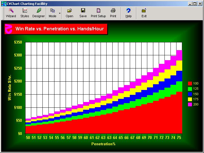
Win Rate vs. Penetration
vs. Hands/Hour
The question was, if you a game has less penetration,
but is faster, will I make as much money. The game was double
deck, H17, DAS. For this I ran 26 sims (actually one CVCX
sim) for penetrations from 50% to 75% in increments of one
card. The chart shows the win rate for each penetration. Five
points are displayed for 100, 125, 150, 175 and 200 hands
per hour. This makes it easy to compare different penetrations
at different speeds. Note, the unit size and betting ramp
are different for each penetration as they are calculated
for maximum bankroll growth. See the chart here: Win
Rate vs. Penetration vs. Hands/Hour
copyright © 2004, QFIT blackjack
card counting products, All rights reserved
|
|


![[link]](http://www.qfit.com/ch12tx.jpg)
![[link]](http://www.qfit.com/ch12wl.jpg)